jupyterhub-pyspark-hdfs-anomaly-detection-taxi-data

To run this demo, your system needs at least:

This demo does not use the Stackable spark-k8s-operator but rather delegates the creation of executor pods to JupyterHub. The intention is to demonstrate how to interact with SDP components when designing and testing Spark jobs: the resulting script and Spark job definition can then be transferred with a Stackable SparkApplication resource. When logging in to JupyterHub (described below), a pod will be created with the username as a suffix, e.g. jupyter-admin. Doing so runs a container hosting a Jupyter Notebook with pre-installed Spark, Java and Python. When the user creates a SparkSession, temporary spark executors are constructed that are persisted until the notebook kernel is shut down or restarted. The notebook can thus be used as a sandbox for writing, testing and benchmarking Spark jobs before they are moved into production.

This demo will:

The Stackable Operator for Apache HDFS will spin up an HDFS cluster to store the taxi dataset in Apache Parquet format. This dataset will be read and processed via PySpark.

Before trying out the notebook example in Jupyter, check if the taxi data was loaded to HDFS successfully:

There should be one parquet file containing taxi trip data from September 2020.

Have a look at the available Pods before logging in (operator pods are left out for clarity, you will see more Pods):

JupyterHub will create a Pod for each active user. In order to reach the JupyterHub web interface, create a port-forward:

Now access the JupyterHub web interface via http://localhost:8080

You should see the JupyterHub login page.

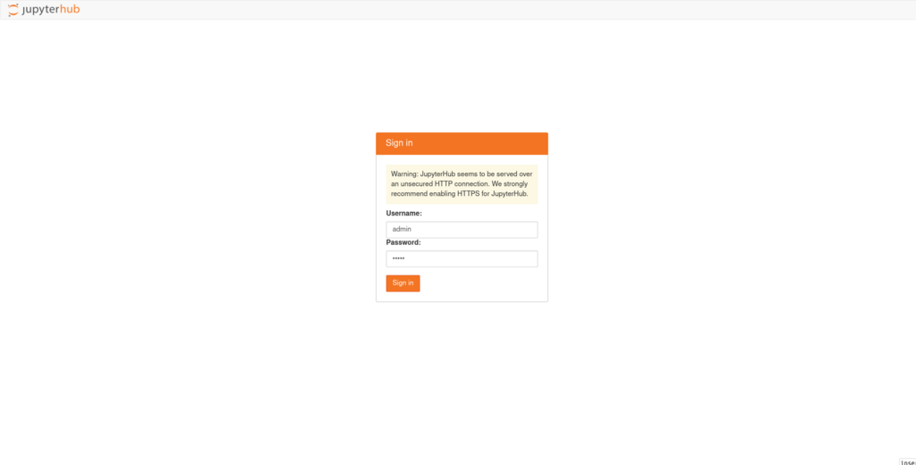
Log in with username admin and password adminadmin. There should appear a new pod called jupyter-admin (operator pods are left out for clarity, you will see more Pods):

You should arrive at your workspace:

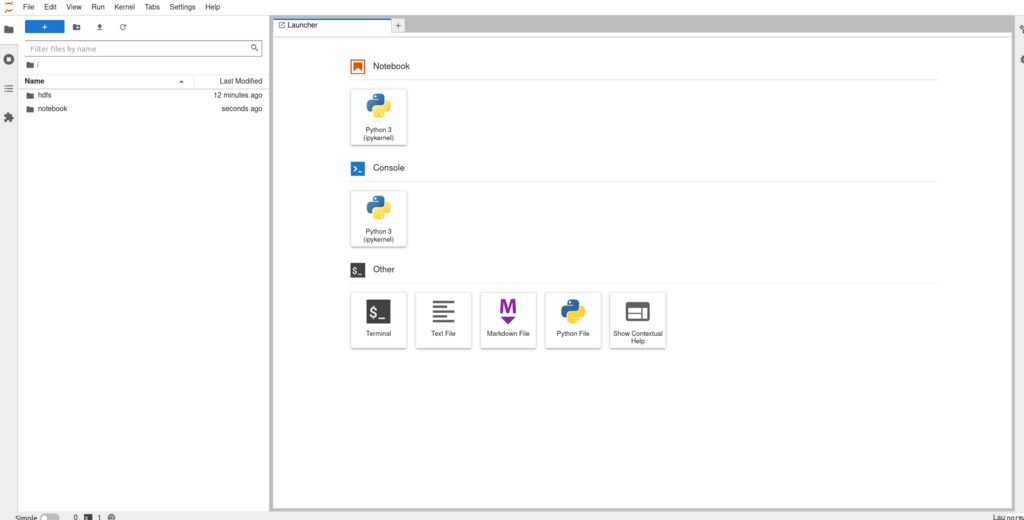
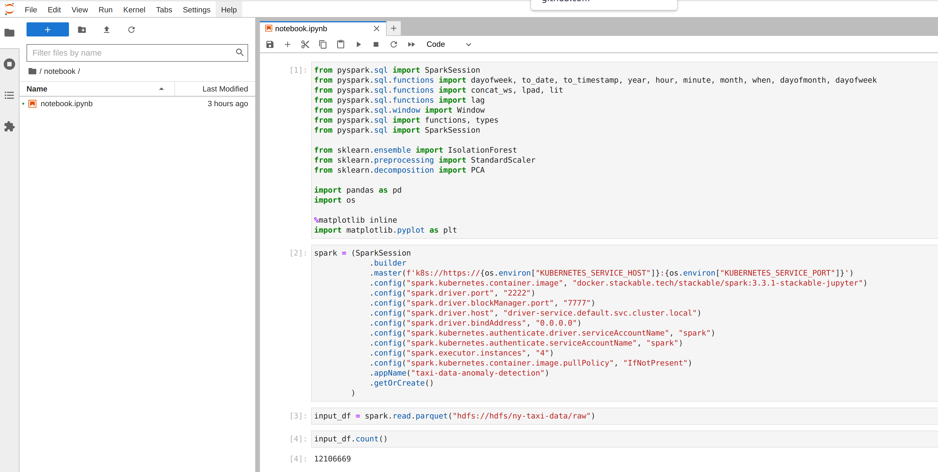
Now you can click on the notebooks folder on the left, open and run the contained file. Click on the double arrow (⏩️) to execute the Python scripts.

You can also inspect the hdfs folder where the core-site.xml and hdfs-site.xml from the discovery ConfigMap of the HDFS cluster are located.

The job uses an implementation of the Isolation Forest algorithm provided by the scikit-learn library: the model is trained and then invoked by a user-defined function (see this article for how to call the sklearn library with a pyspark UDF), all of which is run using the Spark executors spun up in the current SparkSession. This type of model attempts to isolate each data point by continually partitioning the data. Data closely packed together will require more partitions to separate data points. In contrast, any outliers will require less: the number of partitions needed for a particular data point is thus inversely proportional to the anomaly "score".

The notebook shows how to plot the outliers against a particular metric (e.g. "number of rides"):

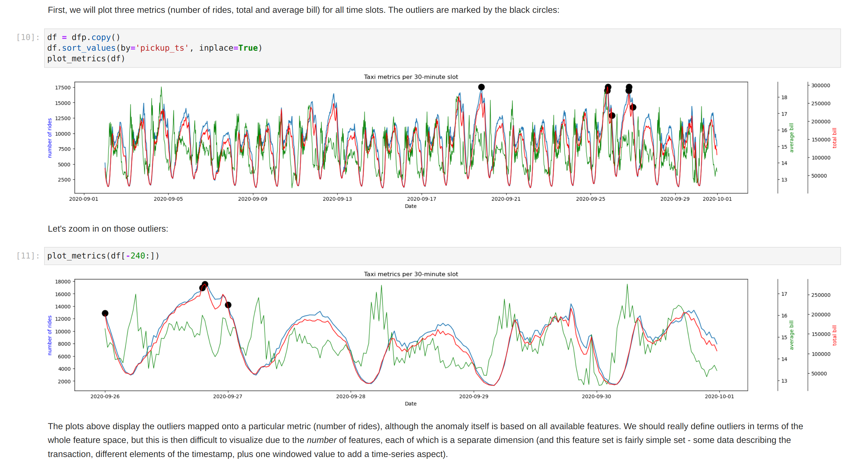
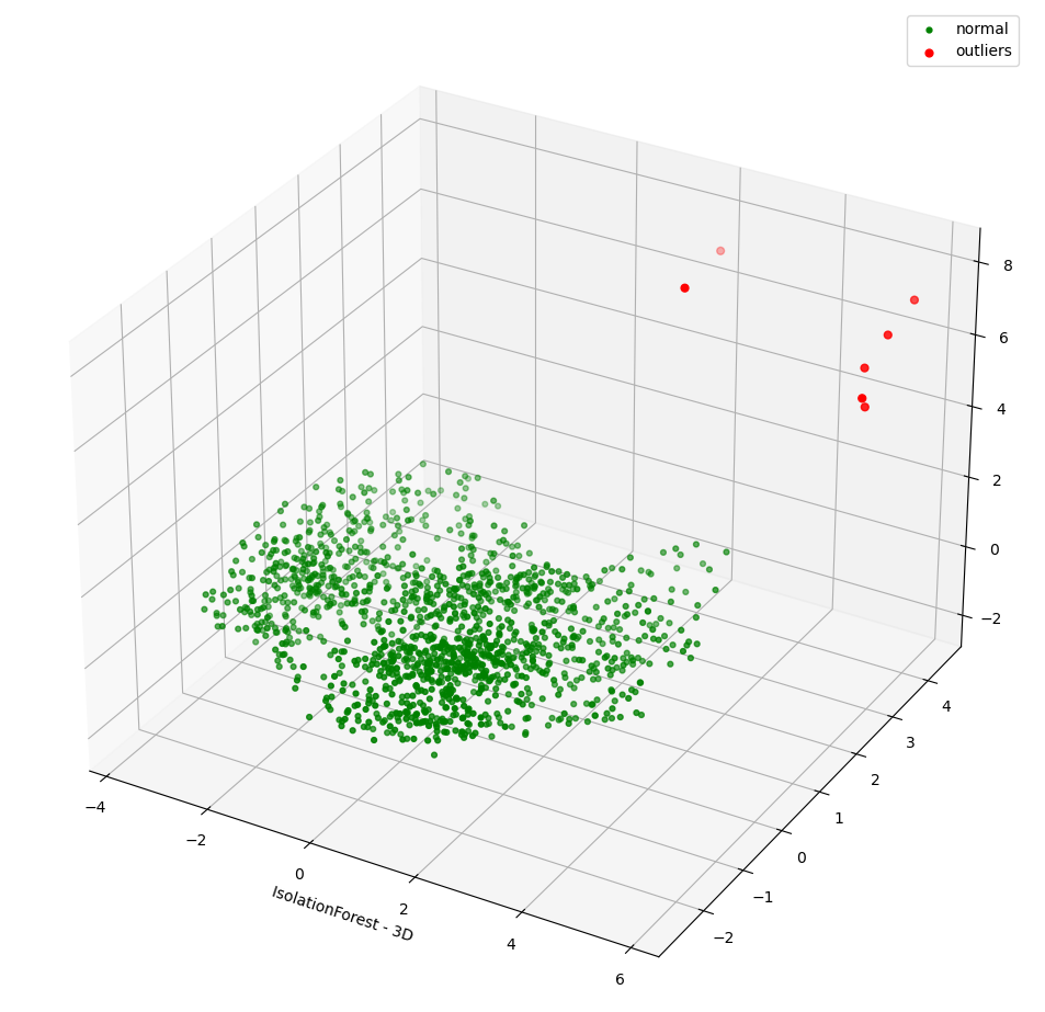
However, this is mainly for convenience - the anomaly score is derived from the entire feature space, i.e., it considers all dimensions (or features/columns) when scoring data, meaning that not only are the results challenging to visualize (how can multidimensional data be represented in only 3-D dimensional space?), but that a root cause analysis has to be a separate process. It would be tempting to look at just one metric and assume causal effects, but the model "sees" all features as a set of numerical values and derives patterns accordingly.

We can tackle the first of these issues by collapsing - or projecting - our data into a manageable number of dimensions that can be plotted. Once the script has finished successfully, plots should be displayed on the bottom that show the same data in 2D and 3D representation. The 3D plot should look like this:

The model has detected outliers even though that would not have been immediately apparent from the time-series representation alone.